Introduction

NOAA satellites sense earth’s surface using six visible light and infrared sensors. The data from these sensors is combined to produce images.

The satellites encode or modulate image data into a 2400 Hz signal. This signal is transmitted to earth via a radio wave between 137 and 138 MHz depending upon which NOAA satellite is received. The format of the transmitted signal is called Automatic Picture Transmission (APT).

Using an antenna and software defined radio, you can record the signal transmitted by a NOAA satellite. See this DIY Satellite Ground Station workshop resource for an accessible set of instructions. Your recording, in the form of a WAV audio file, can be decoded into an image using different methods.

Absolute Value, Cosine and Hilbert/FFT are three methods for decoding or demodulating the WAV file into an image. They operate in slightly different ways, and so will produce different images. Histogram Equalisation increases the contrast of the image.

open-weather apt emerged from a desire to understand the process of decoding APT audio recordings into NOAA satellite images, and a need for an accessible online decoder for new practitioners during open-weather DIY Satellite Ground Station workshops.

open-weather apt is forked from Thatcher’s APT 3000. It is a collaboration between open-weather, Bill Liles NQ6Z and Grayson Earle.

How does a sound become an image?

Recording a NOAA satellite signal using software defined radio produces an audio file. How does this audio file translate into an image?

Let’s first take a look at the format of APT transmission: what are NOAA satellites sending to earth?

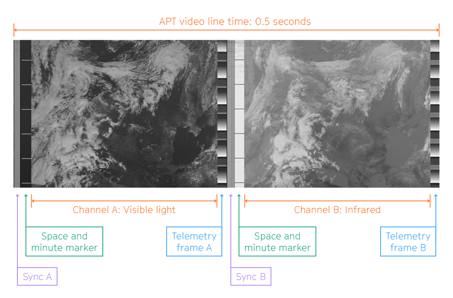
The APT format includes:

• two channels of image data: channel A and channel B
• two sync signals: sync A and sync B
• telemetry data: telemetry frame A and telemetry frame B
• space data and minute markers

One line of information in the APT format (including sync signals, telemetry, space data and channel A/B images) takes 0.5 seconds. This means two full lines of data are transmitted per second.

After listening, you may observe that there is a clear rhythm in the audio. There is a characteristic ‘tick tock’ at regular intervals. There is also a high pitched ‘ring’ or tone that sounds a lot like this.

What are you hearing? The audio file contains three important frequencies: 2400 Hz, 1040 Hz and 832 Hz. These frequencies correspond to specific parts of the APT format. All other frequencies in the audio file are noise caused by your radio environment, your ground station setup or your body.

The three frequencies carry different information:

• 2400 Hz Pixel values (in grayscale) for channel A and B images
• 1040 Hz Channel A sync signal
• 832 Hz Channel B sync signal

We can visualise these frequencies to get a better understanding of how they carry data. The image below (Figure 2) shows the APT signal in a section of an audio recording. (Note: an absolute value function has been applied so that we are only seeing positive values of the signal. A wave normally includes positive and negative values).

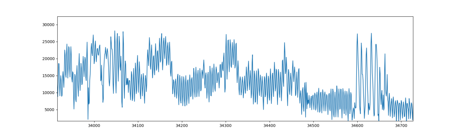
The APT signal is represented by the blue line. The x axis is samples of data. The units of the y axis depend on the programme used to visualise the signal. From 34000 to 34600 samples on the x axis, the ‘level’ or amplitude of the signal changes, yet the frequency remains the same. The different amplitudes can be mapped onto pixel values in grayscale, where black corresponds to a very low value (e.g. 0) and white is a high value.

However, it is not as easy as mapping every value of a wave amplitude onto a pixel value. Depending on the sample rate in which the audio file was recorded, there will be a different number of samples per second. Common audio sample rates are 48000, 44100 and 11025 samples per second.

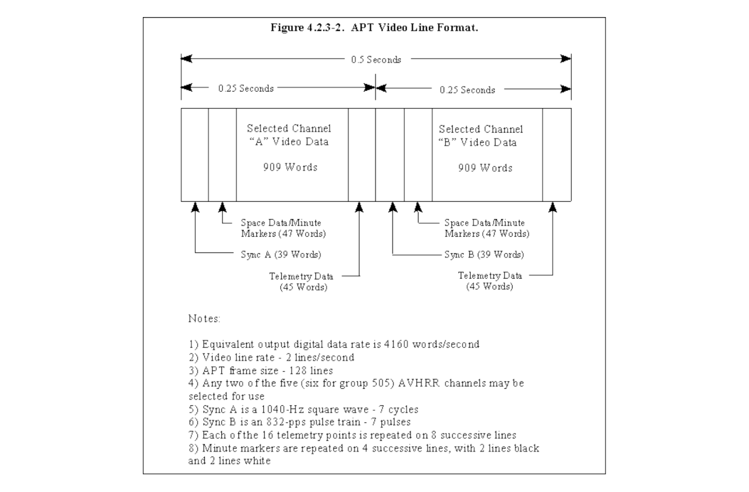
As shown in Figure 3 below, the satellite sends only 909 words’ in one line of Channel A, and 909 ‘words’ in one line of Channel B.

For NOAA, ‘words’ means units of information, or pixels. This means that there are 909 pixels in each line of Channel A and Channel B respectively. One complete line of data, including telemetry, syncs and space data, has 2080 pixels. To determine what the values of these pixels are, it is necessary to downsample the audio file from its original sample rate. open-weather apt accepts audio files at 11025 samples per second, and downsamples this information to 4160 samples per second (2080 pixels per line in 0.5 seconds × 2 = 4160 pixels per second).

Returning to Figure 2, it is possible to identify Sync A. After 34600 samples on the x axis, note that the frequency and amplitude changes: there are seven distinct spikes in the blue line. These seven spikes are the Sync A signal. This signifies the start of a new line of data in the APT format.

Signal strength

The clarity of the satellite image is partly dependent on signal strength. As signal strength decreases, the image quality decreases because it becomes more difficult to distinguish the 2400 Hz amplitude levels to determine the pixel values. When the signal is weaker, the signal to noise ratio is also worse, so determining the correct amplitude might be impossible or not consistent.

A weak signal or a noisy file can also result in a missed channel A sync signal which may produce a slanted image (see Figure 4 below).

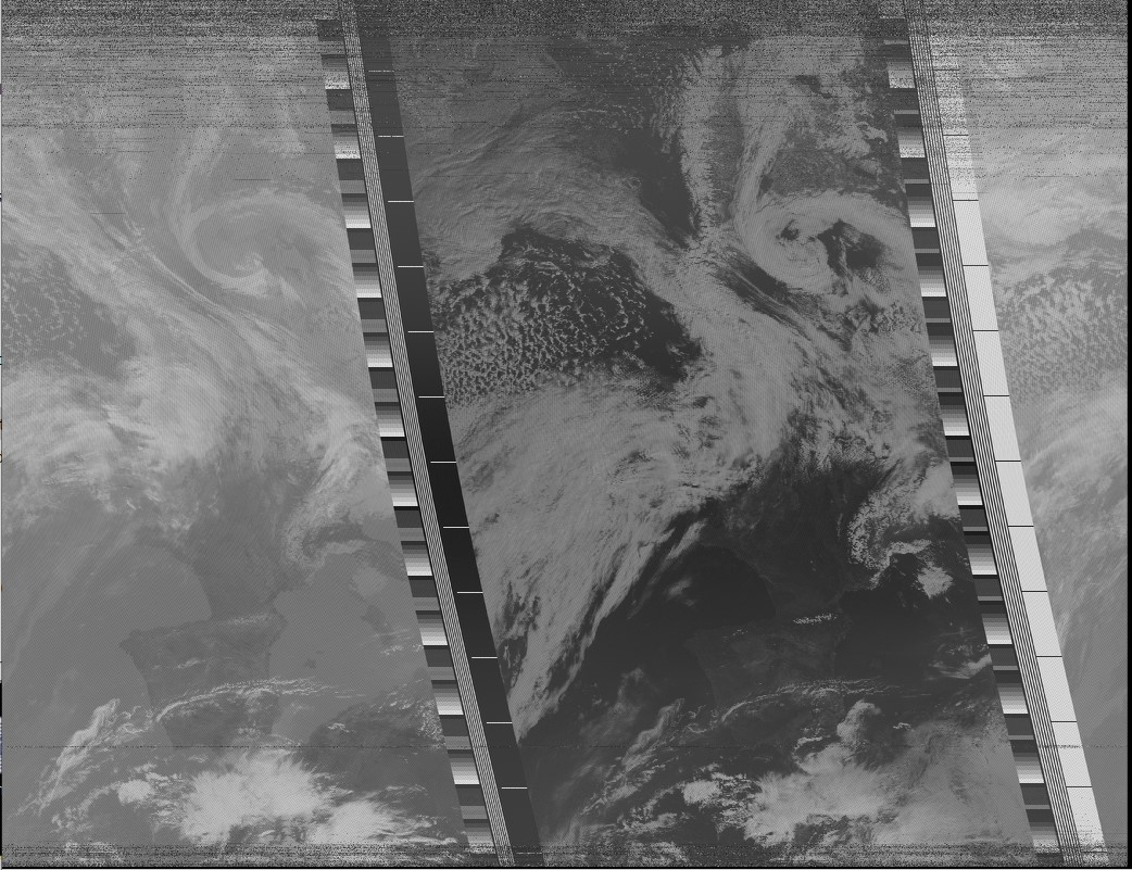
Open-weather apt was designed with first-time satellite signal decoders in mind. Unlike other satellite signal decoders that do not specify where they search for the first ‘sync’ in the audio file, open-weather apt allows you to modify the number of seconds in which the programme searches for the first sync. This means that the programme can more easily find the first sync even when the beginning of the audio file is very noisy.

Demodulation methods

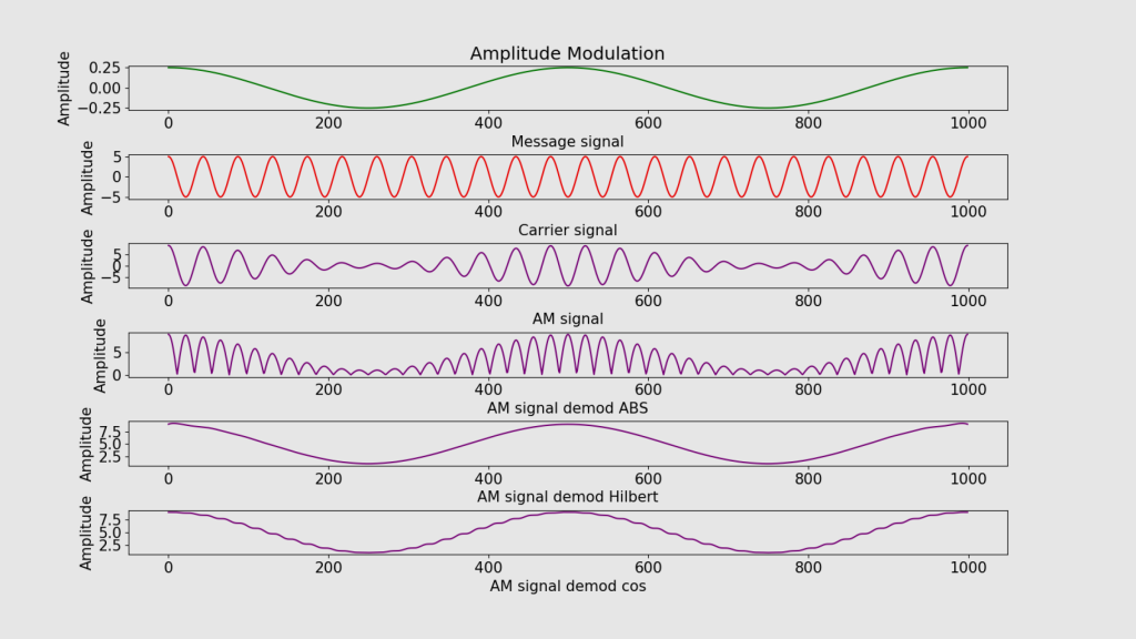
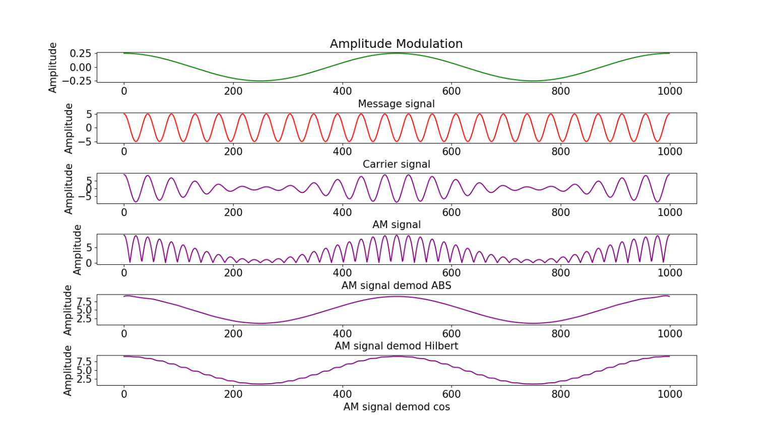
There are several different ways to demodulate the APT signal into an image. The diagram below represents these methods.

The green line is the message signal (we can think of it as the original data transmitted by the satellite). The red line is the carrier signal, and the purple line shows the modulated signal (where the carrier signal has been modulated by the message signal). The demodulation process should retrieve something that is as close to the original message signal as possible.

The three bottom purple lines show the signal demodulated using ABS (Absolute Value); the signal demodulated using the Hilbert FFT method; and finally, the signal demodulated using the law of Cosines.

Absolute Value

This is the simplest and quickest way to decode an audio recording of an APT signal into an image.

A wave, for example a 2400 Hz sine wave, has negative and positive values. If we take the absolute value of all the points in the wave, we end up with only positive values in a time series. After applying a downsampler, we can derive the data for the ‘words’ or pixels in the NOAA satellite image.

Hilbert FFT

This is the most processing-heavy, but most precise, way to decode an audio recording of an APT signal into an image.

We have a time series of samples. First, we turn that time series into what are known as I/Q signals.

There are two ways to do this. One is to use a FIR (Finite Impulse Response filter) with a specific set of coefficients known as a Hilbert Transform. This filter produces the Q time series to go along with the I time series. The other way involves taking the Fast Fourier Transform (FFT) of the input time series, set all the negative frequencies of the transform to zero and then take the inverse Fourier Transform. This is the method that is used in open-weather apt.

Given an I/Q time series, the AM demodulation is the absolute value of each pair of points defined as: abs(I_i, Q_i) = sqrt( I_i * I_i + Q_i * Q_i) where I_i and Q_i are the ith samples of the I/Q time series.

Cosine

This demodulation method is sourced from Martin Bernardi’s code for the open-source satellite signal decoding programme NOAA APT 1.4.0.

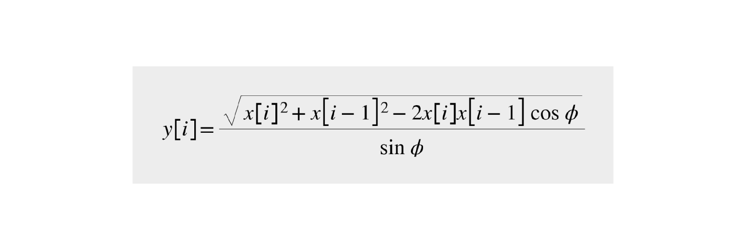
To generate each output sample, we use the current input sample, the previous input sample and the carrier frequency. Note: the sine and cosine functions are computed in radians and not degrees. Theta is 2π times the carrier frequency in Hz divided by the sample rate in samples/sec.

The method uses the following equation:

Increasing image contrast

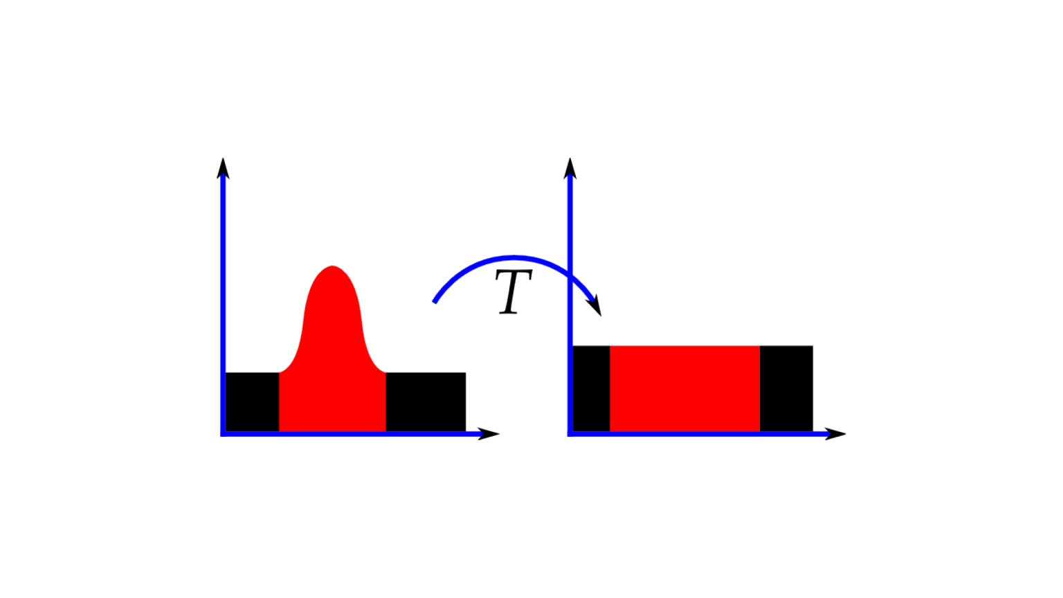
Raw NOAA satellite images often appear grey, low contrast. Histogram equalisation can be applied to increase the global contrast of the image and so reveal details, such as cloud features or the difference between coastline and water. Histogram equalisation effectively spreads out the most frequent pixel brightness values (coloured red in the Figure 7). In other words, it stretches out the intensity range of the image.

Other resources

Go to the Open-weather apt GitHub repository